Introduction
There are generally two types of distortion that loudspeakers produce, time and spectrum distortion. Time and frequency distortions can be directly related to each other, but not always. The ToneBurst program focuses on Energy Decay. Here are some examples:
Time Distortions
- Phase
- Delay
- Energy Decay
Frequency Distortions
- Frequency Response
- Harmonic Distortion
- Intermodulation Distortion
I initially learned about shaped tone burst testing from Sigfried Linkwitz's website 20+ years ago: https://www.linkwitzlab.com/mid_dist.htm
After studying up on burst testing I took it one step further, stepped sweep burst testing. Time analysis of speaker tone burst signals will reveal stored energy released after the input signal has stopped. This stored energy can be caused by the drivers, speaker cabinets, or room.
Here is a program I created to test tone bursts and stepped sweep tone burts. You can read about some of its functions below, it will be expanded soon. If you decide to check it out, please remember that this program is not digitally signed, so your browser will throw a warning when you try to download it. To prevent the warning I would need to pay to get it digitally signed, I don't want to pay to get it signed. The program is free to use, there's no warranty, use at your own discretion. If you decide to use it, all I ask is that you provide attribution back to this website. Suggestions are always welcome, use the contact email in the top menu.
ToneBurst v2.3 — Reference Manual
Overview
ToneBurst generates calibrated tone burst WAV files and analyzes their Energy-Time Curve (ETC) using the Hilbert Transform envelope method. It is designed to measure transient response, decay characteristics, and comparative differences between a Device Under Test (DUT) and a reference recording.
Create a burst or sweep WAV test signal
Play through DUT, record the output
Run analysis to produce ETC graphs
A/B two recordings to measure differences
Browse generated SVG / PNG graphs
The ETC shows how energy decays over time after a tone burst. It is computed using the Hilbert Transform to extract the analytic signal envelope, displayed in dB. A clean transducer shows a sharp peak followed by rapid, smooth decay. Resonances appear as bumps or slow decay after the initial peak.
The DUT (Device Under Test) is the recording through the device being measured. The reference is a direct or known-good recording of the same signal. Overlaying them reveals differences in transient behaviour, energy storage, and decay rate.
The primary comparison metric is |Diff| % — the absolute area difference between the DUT and reference ETC curves, expressed as a percentage of the reference area above the threshold. Lower is better; 0% means the DUT is identical to the reference above the analysis threshold.
Generate
Creates calibrated WAV test signals. Two modes are available: Single Burst generates one tone at a fixed frequency; Sweep generates a series of bursts stepping through a frequency range at a defined octave resolution. Output files are written to the GEN directory.
Generates a single sinusoidal tone burst at the specified frequency. The burst is a short, windowed sine wave at peak amplitude, followed by silence. DTMF markers are embedded before and after the burst so the analyzer can automatically locate it. Output: WAV and optionally SVG PNG graphs.
Generates a sequence of tone bursts stepping from Start Hz to End Hz in 1/N octave steps. Each burst is separated by a silence gap and uniquely identified by DTMF encoding. Designed to be played once through the DUT while recording the output, capturing all test frequencies in a single take.
| Parameter | Mode | Description | Default |
|---|---|---|---|
Frequency (Hz) |
Burst | The centre frequency of the tone burst in Hz. Valid range: 1 Hz – 47 999 Hz. | 1000 |
Start (Hz) |
Sweep | Lowest frequency in the sweep sequence. | 100 |
End (Hz) |
Sweep | Highest frequency in the sweep sequence. | 20000 |
1/N Oct |
Sweep | Frequency resolution. 3 = 1/3 octave steps, 6 = 1/6 octave, etc. Higher values produce more test frequencies. | 3 |
Headroom (dB) |
Both | Peak level below full scale (0 dBFS). 3 dB headroom means the burst peaks at −3 dBFS. | 3 |
Noise (dB below) |
Both | Adds Gaussian pink noise at the specified level below the burst peak. Used to simulate real recording conditions or test SNR performance. | off |
WAV |
Burst | Output a WAV file of the generated signal to the GEN directory. | on |
SVG / PNG |
Burst | Immediately analyze the generated WAV and produce ETC graph output files. | off |
Distortion |
Both | Applies a multi-mode peaking EQ to simulate resonant distortion. Each of 6 modes has independent frequency ratio, Q, gain, window cycles, and delay settings. Enable the checkbox to expand the mode editor. | off |
Analyze
Analyzes a DUT recording against its embedded reference signal. The analyzer auto-detects whether the WAV is a single burst or a sweep using the embedded DTMF markers, then dispatches to the appropriate analysis engine. Output files are written to the IMG directory.
The first DTMF digit embedded in the WAV file identifies the recording type. Digit 1 = single burst; digit 2 = sweep. The analyzer reads this automatically — no manual mode selection is required.
Produces an ETC (Energy vs. Time Curve) graph showing the DUT envelope in magenta and the reference envelope in blue on the same axes. Outputs: SVG PNG
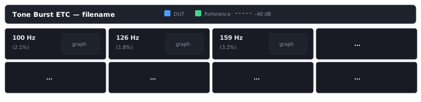
A single frequency-vs-|Diff|% chart covering the full sweep range on a log frequency axis. Shows how the DUT differs from reference at every tested frequency. Y axis range is configurable (default 0–20%).
A grid of small ETC thumbnails, one per test frequency, showing the DUT (magenta) and reference (blue) curves side by side. Useful for quickly spotting which frequencies have abnormal decay.
Individual full-size ETC graphs for each frequency in the sweep, saved as separate files. Equivalent to running burst analysis on every frequency individually.
| Parameter | Description | Default |
|---|---|---|
WAV File |
Path to the DUT recording. Can be in the DUT directory (filename only) or a full path. Use Browse to navigate. | — |
Threshold (dB) |
Analysis threshold in dB below peak. Only signal above this level is included in the area integral. Increase to reduce noise influence; decrease to include more of the tail. | 40 |
Window Cyc |
Analysis window size in periods of the burst frequency. Wider windows capture more of the decay tail; narrower windows focus on the main burst. | 16 |
No Burst Overlay |
Render the ETC graph without the reference overlay curve. Useful when analyzing a recording that has no reference (e.g., a single-channel capture). | off |
Noise Floor |
Measure and display the noise floor of the recording as a horizontal line on the ETC graph. | off |
Set Noise Floor |
Use the measured noise floor as the analysis threshold, overriding the manual Threshold value. Ensures the integral stops at the actual noise level. | off |
ETC Markers |
Overlay peak and −3 dB crossing markers on ETC graphs. Shows the burst peak as a vertical dashed line and the −3 dB half-power points for both DUT and reference. | off |
SVG Sweep Y Min / Max % |
Sets a fixed Y axis range for the SVG Sweep frequency chart. Leave blank for automatic scaling. The default 0–20% range suits most measurements; increase for highly distorted devices. | 0 / 20 |
Compare A/B
Compares two DUT recordings of the same test signal against each other, or against a shared reference. Produces an overlay ETC graph with crosshatch difference shading and quantitative |Diff|% statistics for each recording.
Renders DUT A (magenta) and DUT B (blue) on the same ETC axes, with the shared reference in green dashed. Yellow crosshatch highlights where A exceeds reference; blue crosshatch highlights where B exceeds reference. |Diff| % values for both are printed in the graph subtitle.
Exports per-sample ETC data for both recordings to a CSV file for post-processing in spreadsheet software or other analysis tools.
| Parameter | Description | Default |
|---|---|---|
File A |
First DUT recording WAV file. Must be a burst recording containing an embedded reference signal. | — |
File B |
Second DUT recording WAV file for comparison. Must be from the same test signal as File A. | — |
Label A / B |
Short labels used to identify each recording in the graph legend and CSV header. | A / B |
Threshold (dB) |
Analysis threshold below peak. Identical to the Analyze tab threshold — defines the integration region. | 40 |
Window Cyc |
Analysis window size in periods. Should match the setting used when analyzing individually. | 16 |
SVG Overlay |
Generate the A/B comparison SVG graph with both curves and difference shading. | on |
CSV Export |
Export per-sample ETC values for both recordings to a CSV file. | off |
View
Built-in image browser for SVG and PNG output files. Displays graphs directly in the application window without needing an external viewer. Auto-fits images to window width and supports keyboard navigation through a directory of files.
Choose a folder to browse. All SVG and PNG files in the directory are loaded into the navigation list. The IMG directory is used by default. Files are sorted alphabetically.
Open a specific SVG or PNG file directly. The file's parent directory is automatically loaded for navigation, so you can Page Up / Page Down through neighbouring files after selecting one.
Cycle through all images in the current directory. Works both via the ◀ PgUp / PgDn ▶ buttons and the keyboard Page Up / Page Down keys when the View tab is active.
+ zooms in, − zooms out in 25% increments. Fit restores auto-fit-to-width mode, which also re-applies automatically whenever the window is resized while in fit mode.
Directories
ToneBurst organizes files into three subdirectories relative to the application executable. They are created automatically on first run.
WAV files produced by the Generate tab are saved here. Files are named toneburst_<freq>Hz.wav for bursts and toneburst_sweep_<start>-<end>Hz_1-<N>oct.wav for sweeps.
Place your recorded WAV files here. The Analyze and Compare tabs default their browse dialogs to this directory. Files can be referenced by filename alone if placed here.
All SVG and PNG graphs produced by analysis are saved here. The View tab defaults to browsing this directory. Filenames include the source WAV name and graph type (e.g. _sweep.svg, _mini1.svg, _100Hz.svg).
This help file (tonebursthelp.html) is saved here and can be reopened at any time from the Help button on the Generate, Analyze, or Compare tabs.
Command Line Interface
ToneBurst can be run from the command line for automation and scripting. Run without arguments to launch the GUI, pass a command flag to run headlessly.
# Generate a single burst at 1 kHz
ToneBurst -genburst 1000 -wav

# Generate a sweep from 100 Hz to 20 kHz at 1/3 octave
ToneBurst -gensweep -sweepstart 100 -sweepend 20000 -sweepoct 3

# Analyze a recording (auto-detects burst or sweep)
ToneBurst -analyze DUT\my_recording.wav

# Analyze burst with SVG + ETC markers
ToneBurst -analyze DUT\burst.wav -svg -etcmarkers

# Analyze sweep, all output formats, fixed Y axis 0–10%
ToneBurst -analyze DUT\sweep.wav -svgsweep -svgmini -svgdiscrete -sweepymin 0 -sweepymax 10

# Generate with noise and distortion
ToneBurst -genburst 1000 -wav -headroom 3 -noise 60
| Switch/Flag | Applies To | Description |
|---|---|---|
-genburst <Hz> |
Generate | Generate a single tone burst at the given frequency. |
-gensweep |
Generate | Generate a sweep sequence (requires -sweepstart, -sweepend, -sweepoct). |
-wav |
Generate | Output a WAV file. |
-analyze <file> |
Analyze | Analyze a sweep or burst recording. |
-threshold <dB> |
Analyze | Analysis threshold below peak (default: 40). |
-window <cyc> |
Analyze | Window size in periods (default: 16, minimum: 4). |
-noisefloor |
Analyze | Measure and show noise floor on graphs. |
-setnoisefloor |
Analyze | Use measured noise floor as analysis threshold. |
-etcmarkers |
Analyze | Show peak and −3 dB markers on ETC graphs. |
-headroom <dB> |
Both | Peak headroom below 0 dBFS (default: 3). |
-noise <dB> |
Both | Add Gaussian pink noise at dB below peak. |
-svg / -png |
Burst | Output SVG / PNG graph for burst analysis. |
-svgsweep / -pngsweep |
Sweep | Output SVG / PNG frequency sweep chart. |
-svgmini / -pngmini |
Sweep | Output SVG / PNG mini ETC grid. |
-svgdiscrete / -pngdiscrete |
Sweep | Output individual SVG / PNG ETC graphs per frequency. |
-sweepstart <Hz> |
Sweep | First frequency in sweep sequence. |
-sweepend <Hz> |
Sweep | Last frequency in sweep sequence. |
-sweepoct <N> |
Sweep | 1/N octave step resolution. |
-sweepymin <%> |
Sweep | Fixed Y axis minimum for sweep chart (default: auto). |
-sweepymax <%> |
Sweep | Fixed Y axis maximum for sweep chart (default: auto). |
WAV Output File Structures
Single Burst & Burst Sweep signal format specification
Single Burst WAV
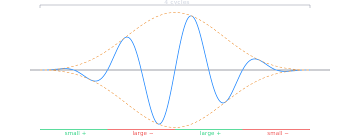
A single 4-cycle Blackman-windowed tone burst at one target frequency, framed by DTMF-encoded metadata and band-limited PRN sync markers.
| # | Region | Duration | Description |
|---|---|---|---|
| 1 | Silence | 1000 ms | Lead-in silence |
| 2 | DTMF Encoding | 6 × 75 ms | Type-prefixed frequency: 1FFFFF — digit 1 identifies burst type, followed by 5-digit zero-padded frequency (e.g. 101000 for 1000 Hz). Each digit is a 50 ms dual-tone + 25 ms gap at 25% peak amplitude, Hann-windowed. Band selected automatically by test frequency. |
| 3 | Silence | 1000 ms | Gap after DTMF |
| 4 | Start PRN Sync | 100 ms | Band-limited PRN — sum of sinusoids at 1/12-octave spacing from 100 Hz to 20 kHz, with 1/√f pink weighting and deterministic LCG phases. High-pass filtered via 2-pole Butterworth at freq/2 (capped 2 kHz). 50% peak amplitude, 10 ms Hann fade in/out. |
| 5 | Silence | 1000 ms | Gap after PRN |
| 6 | Tone Burst | 4 cycles | 4-cycle Blackman-windowed sine burst at the target frequency, plus optional distortion tail from multi-mode peaking EQ. |
| 7 | Silence | 1000 ms | Gap before noise floor region |
| 8 | Noise Floor | 1000 ms | Silent region used for noise floor measurement |
| 9 | End PRN Sync | 100 ms | Same band-limited PRN signal as start, with Hann fade in/out |
| 10 | Silence | 500 ms | Trail-out silence |
Burst Sweep WAV
Multiple 4-cycle bursts at logarithmically-spaced frequencies, sharing the same DTMF-first framing structure as the single burst.
| # | Region | Duration | Description |
|---|---|---|---|
| 1 | Silence | 1000 ms | Lead-in silence |
| 2 | DTMF Encoding | 17 × 75 ms | Type-prefixed sweep parameters: 2SSSSSEEEEEOOIIII — digit 2 identifies sweep type, followed by 5-digit start freq, 5-digit end freq, 2-digit octave division, 4-digit interval (ms). Band selected by sweep start frequency. |
| 3 | Silence | 1000 ms | Gap after DTMF |
| 4 | Start PRN Sync | 100 ms | Band-limited PRN — HP filtered via 2-pole Butterworth at startFreq/2 (capped 2 kHz). 50% peak amplitude, 10 ms Hann fade in/out. |
| 5 | Silence | 1000 ms | Gap after PRN |
| 6 | Burst Region | interval × count | Repeating fixed-length slots. Interval = 25× the period of the lowest frequency, minimum 250 ms. Each slot has 500 silent samples then the burst. Frequencies step by 21/OctDiv from start to end. |
| 7 | Silence | 1000 ms | Gap before noise floor region |
| 8 | Noise Floor | 1000 ms | Silent region used for noise floor measurement |
| 9 | End PRN Sync | 100 ms | Same band-limited PRN signal as start, with Hann fade in/out |
| 10 | Silence | 500 ms | Trail-out silence |
Key Differences from Single Burst
- DTMF type prefix
2(sweep) vs1(burst) — auto-detected by analyzer - DTMF payload encodes sweep parameters (17 digits) instead of a single frequency (6 digits)
- PRN is band-limited to the sweep start frequency range
- Burst region contains many fixed-interval slots instead of one burst
DTMF Type Prefix
The first DTMF digit identifies the file type, allowing the analyzer to auto-detect and route to the correct analysis path.
| Prefix | Type | Format | Total Digits |
|---|---|---|---|
| 1 | Single Burst | 1FFFFF |
6 |
| 2 | Burst Sweep | 2SSSSSEEEEEOOIIII |
17 |
DTMF Band Selection
The DTMF band is chosen automatically to avoid overlap with the test frequency. Each digit is encoded as a simultaneous pair of tones — one from the Low Group (row) and one from the High Group (column).
Digit → Row / Column Mapping
Each digit 0–9 selects one frequency from the Low Group (row index) and one from the High Group (column index). The two tones are transmitted simultaneously for 50 ms.
| Digit | Row Index | Col Index | Example (MID Band) |
|---|---|---|---|
| 0 | 3 | 1 | 3760 Hz + 5340 Hz |
| 1 | 0 | 0 | 2800 Hz + 4840 Hz |
| 2 | 0 | 1 | 2800 Hz + 5340 Hz |
| 3 | 0 | 2 | 2800 Hz + 5900 Hz |
| 4 | 1 | 0 | 3080 Hz + 4840 Hz |
| 5 | 1 | 1 | 3080 Hz + 5340 Hz |
| 6 | 1 | 2 | 3080 Hz + 5900 Hz |
| 7 | 2 | 0 | 3400 Hz + 4840 Hz |
| 8 | 2 | 1 | 3400 Hz + 5340 Hz |
| 9 | 2 | 2 | 3400 Hz + 5900 Hz |
PRN Sync Signal
The sync signal is a sum-of-sinusoids — a deterministic, reproducible waveform constructed by adding together a large number of sine waves simultaneously. Here's each stage in detail.
Sweep Generation (-gensweep)
- Frequency grid — 1/12-octave spacing starting at 100 Hz, each successive frequency is multiplied by 2^(1/12) ≈ 1.0595, the same interval as a semitone in musical pitch. This continues up to 20 kHz, producing approximately 96 frequencies covering the full audio range. Using logarithmic spacing means the frequencies are perceptually evenly spread — as many components cover 100–200 Hz as cover 10–20 kHz — which gives the signal a noise-like texture across the whole band rather than clustering energy at the low end.
- The sum-of-sinusoids controls exactly which frequencies are present and at what amplitude, you can shape the spectrum to match the measurement context and guarantee that the generator and detector always use bit-for-bit identical reference waveforms regardless of platform or runtime. The cross-correlation between the recorded signal and the known reference then has a sharp, unambiguous peak at the correct sync position even if the recording is bandlimited or frequency-coloured by the device under test.
- Phase randomisation — All those sine waves starting at zero phase would produce a huge coherent spike at t=0. To prevent that, each sinusoid is given a pseudo-random starting phase. The phases are generated by the classic glibc Linear Congruential Generator. The output of each step is mapped to a phase in the range 0–2π. All that's needed is that the phases are sufficiently spread out to break the coherent spike, and that the exact same phases are reproduced every time the code runs, so the generator and detector always agree on the reference waveform.
- Pink Noise amplitude weighting 1/√f — Each sinusoid is scaled by √(refFreq / f), where refFreq is the lowest frequency (100 Hz). This means the 100 Hz component has full amplitude (scale = 1.0), the 200 Hz component has scale ≈ 0.707, the 1 kHz component has scale ≈ 0.316, and the 20 kHz component has scale ≈ 0.071. This is a pink weighting — amplitude falls at 3 dB per octave, which makes the power spectrum flat on a per-octave basis. Without this, the higher frequencies would dominate (white noise) the signal energy and cross-correlation would be biased toward low-frequency content in the recording.
- High-pass filtering - The full-bandwidth signal is then filtered with a 2nd-order Butterworth high-pass at half the lowest burst frequency (capped at 2 kHz). This ensures the PRN doesn't overload a driver, especially small mids and tweeters. For a 1 kHz burst the PRN is high-passed at 500 Hz; for a 100 Hz sweep start it would be high-passed at 50 Hz but the 2 kHz cap applies in practice for any higher frequency tests
DUT Analysis (-analyze)
- The analysis pipeline has six distinct step that apply identically whether processing a single burst or a sweep. The sweep simply iterates steps 4–6 once per frequency.
- Step 1 Reading the WAV File — The WAV is read into memory and scanned in 10 ms energy windows. The first window that exceeds 10× the RMS noise floor (or 50,000 counts absolute minimum) is flagged as the DTMF start. A Goertzel filter then reads just the first DTMF digit across all three frequency bands (LOW/MID/HIGH) simultaneously and picks the band with highest total power. Digit 1 → burst and Digit 2 → sweep. This determines which analysis path runs next.
- Step 2 DTMF Parameter Decoding — The full digit string is decoded using the Goertzel algorithm at the known symbol timing (50 ms tone, 25 ms gap per digit). Every possible band is tried and the one producing the highest total energy across all digits wins. Burst (1FFFFF): 6 digits → frequency extracted as a 5-digit integer. If this fails, FFT is used as fallback. Sweep (2SSSSSEEEEEOOIIII): 17 digits → start frequency, end frequency, octave resolution, and burst interval in ms are all extracted. These values completely describe the test — no external parameters are needed.
- Step 3 PRN Sync and Clock Drift Correction — A reference PRN signal is generated in software using the same function as the genenerate tab. This is cross-correlated against the recording to locate the start PRN precisely. Two-pass correlation: First pass steps every 100 samples across a ±200 ms search window around the expected position for speed. Second pass does a sample-by-sample refinement ±10 samples around the coarse peak. The sub-sample position is resolved by fitting a parabola to the three highest correlation values — sub-sample function returns a fractional sample offset so the PRN is located to better than one sample precision. The End PRN is then found by the same process, searching the second half of the file. With both PRN positions known sub-sampled precisely:
- measuredSpan = endPRN_precise − startPRN_precise
- expectedSpan = known from DTMF (PRN + silence + bursts + silence + noise floor)
- driftRatio = measuredSpan / expectedSpan
- driftPPM = (driftRatio − 1) × 1,000,000
- If drift exceeds 0.5 PPM the entire recording is resampled by driftRatio using windowed sinc interpolation (DSPHelper.Resample), and all sample offsets are recalculated. If drift exceeds 1000 PPM (implausible — different clocks or wrong file) it is discarded. This makes burst timing precise even when the playback and recording devices have independent clocks.
- Step 4 Noise Floor Measurement — If requested, the 1-second silence window immediately before the end PRN is used. The peak absolute sample value in that window is expressed relative to 0 dBFS — this is the noise floor in dBFS. For each individual burst analysis it is then expressed relative to the burst's own peak, giving a burst-relative noise floor in dB. If -setnoisefloor is active, this value replaces the manually set threshold for area integration.
- Step 5 Per Burst Extraction and ETC Computation — For each burst slot (sweep: once per frequency; single burst: once.) The interval window is sliced from the drift-corrected recording and the burst is extracted. The first 500 samples (Burst Lead-In) are silent pre-burst padding, deliberately included because the Hilbert transform needs silence before the burst onset to avoid edge effects. Window length is 500 + WindowPeriods × samplesPerCycle — defaulting to 16 periods, extended to ensure the Windowed/Discrete Hilbert Transform (DHT) has full support at every sample.
- Peak location: A frequency-adaptive RMS window, 4-cycle width, is slid across the interval to find the burst peak position. Silent intervals (below 0.1% of full scale) are skipped.
- Reference generation: A mathematically perfect 4-cycle Blackman-windowed burst at the nominal frequency is synthesised and placed at sample offset 500 within an array of the same length as the DUT window. This is the ideal reference — no room acoustics, no recording chain, just the pure waveform.
- Discrete Hilbert Transform envelope: Both DUT and reference windows are passed to the envelope. The DHT is a windowed FIR approximation of the ideal 2/(πk) impulse response, Blackman-windowed to suppress sidelobes, with a radius of at least 8 periods of the burst frequency. The input is zero-padded by half-width on both sides so the convolution is accurate at all positions. At each sample, the imaginary part (Hilbert output) and real part (original signal minus DC) form a complex pair; the magnitude is √(real² + imag²). This gives the instantaneous amplitude envelope. The result is converted to dB relative to peak and clamped to a −60 dB floor.
- Step 6 |Diff| % Computation — Both envelopes are converted back to linear amplitude for integration. For each consecutive sample pair where at least one envelope is above the threshold, the absolute difference is computed and the area under it is integrated using the trapezoidal rule.
- diffArea += 0.5 × (|DUT[i] − REF[i]| + |DUT[i+1] − REF[i+1]|) × dt
- The DUT area alone is computed the same way (against zero). The |Diff| % metric is: |Diff| % = (diffArea / refArea) × 100
- This expresses how much the DUT's energy-time behaviour deviates from the ideal reference, as a fraction of the reference's own energy above the threshold. A perfect transducer scores 0 %. A device with strong resonant ringing scores higher — there is no upper bound to how badly a device can behave, but the value is capped at 200 % in the code to prevent chart scaling problems.
Sweep Burst Interval
Each burst in the sweep occupies a fixed-length interval. The first 500 samples are guaranteed silent, providing a clean pre-burst padding zone for the Hilbert kernel in the analyzer.
Example: for a 100 Hz–20 kHz sweep, interval = max(250, 25 / 100 × 1000) = 250 ms = 24,000 samples at 96 kHz.
Analysis Windowing
Both burst and sweep analyzers extract a time-domain window around each burst for ETC (Energy Time Curve) analysis via Hilbert transform. The window must include enough silent padding before the burst for the Hilbert kernel to operate without edge truncation.
Single Burst Window
The single burst analyzer locates the burst via PRN sync correlation, then extracts a window centered on the burst peak. The window size is based on the number of analysis periods (default 16) plus extra room for filter delay and ringing tail.
Sweep Burst Window
The sweep analyzer extracts each burst's fixed-length interval starting from the interval boundary. The 500-sample silent lead-in provides guaranteed Hilbert padding regardless of frequency. The window starts at sample 0 of the interval.
ETC Analysis & Oversampling
The ETC (Energy Time Curve) is computed via Hilbert transform at the native 96 kHz sample rate for maximum waveform fidelity. The resulting dB envelope is then oversampled to 768 kHz (8×) for sub-sample alignment precision and smooth SVG rendering.
Processing Pipeline
Why Oversample the Envelope, Not the Waveform?
The Hilbert transform produces the smoothest, most accurate envelope when operating on the original integer samples at the native sample rate. Upsampling the waveform before the Hilbert introduces sinc interpolation artifacts (ripple near transitions) that the kernel picks up as spurious envelope features. By contrast, the dB envelope is a smooth, slowly-varying curve that oversamples cleanly with simple interpolation.
| Stage | Sample Rate | Purpose |
|---|---|---|
| Hilbert transform | 96 kHz | Analytic signal envelope from original waveform — no interpolation artifacts |
| Envelope oversample | 768 kHz (8×) | Sub-sample precision for −3 dB alignment and area integration |
| Fractional shift | 768 kHz | Windowed sinc interpolation aligns DUT left −3 dB crossing to REF |
| |Diff| area | 768 kHz | Trapezoidal integration of |DUT − REF| above threshold, reported as ms² and % |
Alignment Method
DUT and REF envelopes are aligned by their left (rising) −3 dB crossing point. This edge is unaffected by tail ringing or distortion, giving a clean onset alignment. The shift is computed at 768 kHz resolution (1.3 µs precision) and applied via windowed sinc interpolation on the oversampled envelope.
ETC Output Layout
Tone Burst Bandwidth
The bandwidth of a tone burst is determined by its duration, not its frequency. For a 4-cycle burst the duration is T = 4 / f and the approximate −3 dB bandwidth is BW ≈ f / 4 — roughly 25% of the center frequency (±12.5%).
The Blackman window reduces spectral leakage (sidelobes ≈ −58 dB down) but slightly widens the main lobe, so the actual −3 dB bandwidth is closer to f / 3.5 or about 29% of center frequency.
| Frequency | Duration | Bandwidth (−3 dB) |
|---|---|---|
| 100 Hz | 40 ms | ~25 Hz |
| 1 kHz | 4 ms | ~250 Hz |
| 10 kHz | 0.4 ms | ~2.5 kHz |
| 20 kHz | 0.2 ms | ~5 kHz |
This is why tone bursts are useful for transient / time-domain analysis — they are short enough to measure time-domain behavior but have enough bandwidth to excite the system meaningfully. The trade-off is that you cannot isolate a single frequency the way you would with a long steady-state sine wave.
For speaker measurements, this bandwidth is actually desirable since it shows how the speaker responds to transient signals across a range of frequencies simultaneously, which is more representative of real audio content (music, speech) than pure tones.
4-Cycle Blackman-Windowed Reference Burst
Optimal Octave Spacing
For adjacent burst spectra to "just touch" at their −3 dB points, we need the upper −3 dB edge of one burst to meet the lower −3 dB edge of the next.
Bandwidth ≈ 29% of center frequency (±14.5%). Upper −3 dB edge: f × 1.145. Lower −3 dB edge: f × 0.855.
Derivation
f₂ / f₁ = 1.145 / 0.855 = 1.339
21/n = 1.339 → 1/n = log₂(1.339) = 0.421 → n ≈ 2.37
| Setting | Step Ratio | Coverage |
|---|---|---|
-sweepoct 2 (½ octave) |
1.414 | Slight gaps between bursts |
| Optimal ≈ 1/2.4 octave | 1.339 | Spectra just touch |
-sweepoct 3 (⅓ octave) |
1.260 | Slight overlap (~6%) |
Since -sweepoct takes integers, use -sweepoct 3 or higher for continuous frequency coverage without gaps.
Parabolic Interpolation for Sub-Sample PRN Detection
Test Signal Structure

The Problem: Integer Sample Resolution
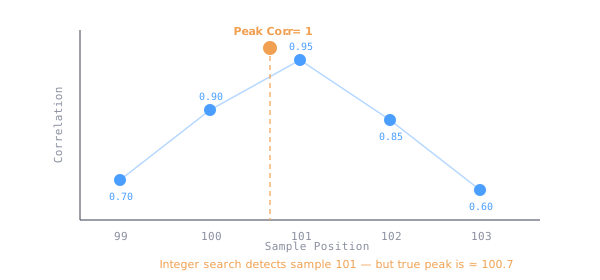
Cross-correlation finds where the PRN best matches, but only at integer sample positions. The true peak of the correlation function almost always falls between samples. A 1-sample error in a 770,400-sample span produces a 1.3 PPM apparent drift.
The Solution: Fit a Parabola
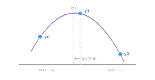
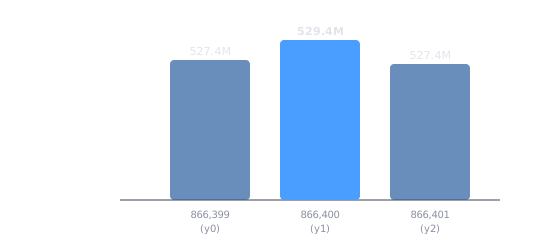
A parabola closely approximates the correlation peak. We use the three samples surrounding the integer maximum — y0, y1 (the peak), and y2 — to calculate where the true peak lies.
The Math
For a parabola passing through points at x = −1, 0, +1 the vertex (peak) occurs at:
Real Example (End PRN Detection)
y0 (lag−1) :  527,410,999
y1 (lag peak): 529,429,464   ← highest correlation
y2 (lag+1) :  527,361,859
y0 − y2          = 49,140
y0 − 2·y1 + y2  = −4,086,070
δ = 49,140 / (2 × −4,086,070) = −0.006013
Integer position  : 866,400
Sub-sample offset : −0.006013
━━━━━━━━━━━━━━━━━━━━━━━━━━━━━━━
Precise position  : 866,399.993987
Precision Improvement
Start PRN: 96000
End PRN: 866400
Span: 770,400 samples
Error: ~1 sample
Drift: ~1.3 PPM
Start PRN: 96000.00513
End PRN: 866399.993987
Span: 770,399.988857
Error: 0.011 samples
Drift: ~0.014 PPM
| Detection Method | Resolution | Min Detectable Drift |
|---|---|---|
| Integer only | 1 sample | ~1.3 PPM |
| Parabolic interpolation | ~0.01 sample | ~0.013 PPM |
Typical consumer audio drift is 20–100+ PPM; professional gear is 1–20 PPM. With parabolic interpolation we can accurately measure even professional-grade clock accuracy.
|Diff| % Metric
The |Diff| % metric compares the Energy Time Curve (ETC) of the Device Under Test (DUT) to an ideal 4-cycle Blackman-windowed reference burst. It measures how much the burst "spreads" or "rings" compared to the ideal.
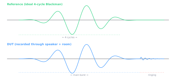
Step 1 — Record the Signals
The reference is the ideal 4-cycle Blackman burst. The DUT signal is recorded through the speaker and room, and may show additional ringing after the main burst.
Step 2 — Compute ETC (Envelope via Hilbert Transform)
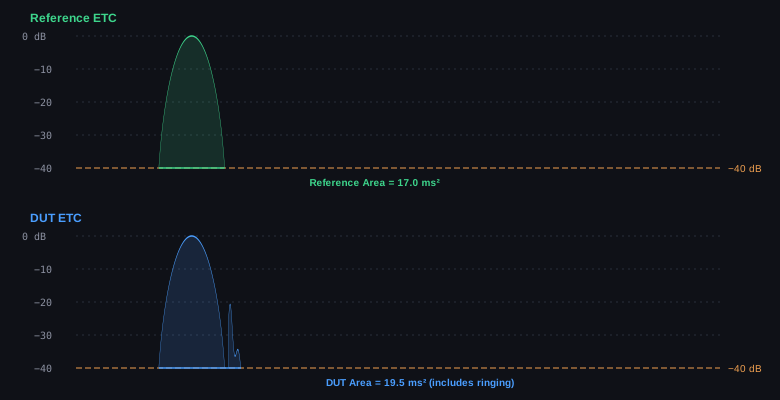
The Hilbert Transform extracts the amplitude envelope, which is then converted to dB scale (0 dB = peak).
Step 3 — Calculate Area Above −40 dB Threshold
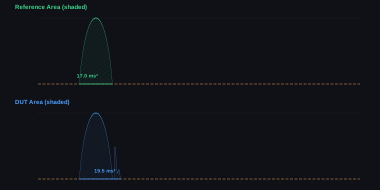
We integrate the linear envelope (not dB) above the −40 dB threshold. The shaded regions below represent the areas being compared.
Step 4 — Calculate |Diff| %
= |19.5 − 17.0| / 17.0 × 100% = 2.5 / 17.0 × 100% = 14.7%
Visual Summary
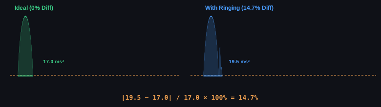
Interpretation Guide
| |Diff| % | Rating | Interpretation |
|---|---|---|
| 0–5% | Excellent | Minimal ringing or resonance |
| 5–15% | Good | Some coloration |
| 15–30% | Fair | Noticeable resonance |
| 30–50% | Poor | Significant ringing |
| >50% | Bad | Severe resonance issues |
Speaker resonance (cone continues moving after signal stops), room reflections (sound bouncing back to microphone), cabinet vibrations (enclosure ringing), and port turbulence (in ported speakers).
Noise Floor Measurement
The noise floor is measured from a dedicated 500 ms silence window located just before the End PRN marker.
Measurement Window Location
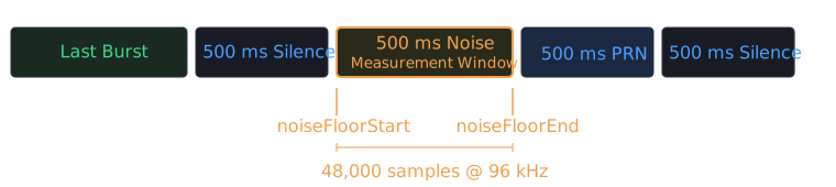
Step 1 — Locate the Window
noiseFloorSilence    = SampleRate × 0.500    # 48,000 samples at 96 kHz
noiseFloorEndSample  = endPrnPosition
noiseFloorStartSample = endPrnPosition − noiseFloorSilence
Step 2 — Calculate RMS
RMS (Root Mean Square) measures the average power of the signal in the noise window.
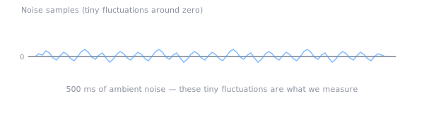
Step 3 — Convert to dBFS
Convert the RMS value to decibels relative to full scale (maximum possible digital value).
For 24-bit audio: Full Scale Max = 8,388,607 (2²³ − 1)
Example:  RMS = 3,340
dBFS = 20 × log₁₀( 3,340 / 8,388,607 )
     = 20 × log₁₀( 0.000398 )
     = 20 × (−3.4)
     = −68 dBFS
Step 4 — Per-Burst Relative Noise Floor
For each burst's mini ETC graph, the noise floor is calculated relative to that burst's peak amplitude, giving the signal-to-noise ratio for that specific frequency.
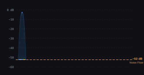
Example: 20 × log₁₀( 3,340 / 6,700,000 ) = 20 × log₁₀( 0.000499 ) = −66 dB
Two Different Noise Floor Values
"Noise Floor: −58.1 dBFS (measured from silence window)"
Measured relative to full scale (0 dBFS). Same value for the entire file. Tells you the actual noise level.
Orange dashed line at −XX dB on each mini ETC graph.
Measured relative to each burst's peak amplitude. Different per burst (lower freq = higher amplitude). Shows SNR for that burst.
Captures system noise without signal interference. Located after all bursts so no burst energy leaks in. 500 ms provides enough samples for a stable RMS measurement. Positioned before the End PRN so the PRN doesn't corrupt the measurement.
Noise sources captured: ADC quantization noise, preamp/mic noise, environmental noise (room, HVAC, etc.), and electromagnetic interference.